Intro to SymPy

SymPy is a Python library for symbolic mathematics. We can use it to solve differential equations, simplify algebraic operations, evaluate integrals and more. SymPy give us exact symbolic answers instead of numerical approximations. You can check SymPy documentation here.

Getting started

The first thing we need to do is to install the SymPy library,

%pip install sympy 

Requirement already satisfied: sympy in /Users/alexandre/.local/lib/python3.9/site-packages (1.12)
Requirement already satisfied: mpmath>=0.19 in /Users/alexandre/.local/lib/python3.9/site-packages (from sympy) (1.3.0)
Note: you may need to restart the kernel to use updated packages.

SymPy is not a built-in module so every time you start a new notebook on Google Colab you need to run the pip command above.

After installing we need to import the library,

import sympy as sy 
sy.init_printing()

import sympy as sy loads in the SymPy library for us to use. We give a shorthand name sy (could be any other name ), so every time we call something from SymPy, we use sy.. This helps to keep things organized.

sy.init_printing() gets the output to be displayed as nicely formatted mathematics.

We can check the difference between using a built-in Python function and the SymPy library by checking this example to compute square roots,

import math 
math.sqrt(8)

Here we got tan approximate result since it can’t be represented by a finite decimal. If all we cared about was the decimal form of the square root of 8, we would be done.

But when we use symbolic computation like SymPy, square roots of numbers the are not perfect squares are left unevaluated by default,

sy.sqrt(8)

More interesting examples

In SymPy variables are defined using symbols,

from sympy import symbols
x,y = symbols('x y')
expression = x + 2*y 
expression

We can play around and see that if we subtract x from the current expression,

expression - x 
#expression 

automatically canceling x with -x.

We can also represent functions in SymPy. For example, let’s represent \(f(x) = x^3 + x^2 + 10\)

f = x**3 + x**2 + 10 
f 

It is important to notice that this is not an actual Python function, described in the previously, rather a symbolic representation of a function. Therefore, to evaluate f for different values we use the subs() function,

f.subs(x,4)

Limits

With SymPy we can evaluate limits symbolically using the limit() function, which has the following syntax,

sy.limit(expression,variable,value)

expression is the function whose limit we are trying to find. variable is the variable with respect we are taking the limit. value is the value the variable is approaching.

To compute one-sided limits, we can add a fourth argument to the function, either a + or - for a right or left hand limit.

For example, let’s evaluate \( \lim_{x \rightarrow 0} \frac{sin(x)}{x}\),

limit = sy.limit(sy.sin(x)/x , x , 0)
limit

And when \(x\) is approaching \(\infty\),

limit = sy.limit(sy.sin(x)/x , x , sy.oo)
limit

Derivatives

We can take derivatives with the diff() function. Given a function \(\sin(x)e^x\), its derivative with respect to \(x\) is,

f = sy.sin(x)*sy.exp(x)
d_x = sy.diff(f,x)
d_x

We can change the variable with respect to we are differentiating,

d_y = sy.diff(sy.sin(x)*sy.exp(x),y)
d_y 

The diff() function can also compute higher order derivatives. Given \(f(x) = \sin(x)\)

f = sy.sin(x)
df_dx = sy.diff(f,x)
df2_dx2 = f.diff(x,x) # second derivative
df3_dx3 = f.diff(x,x,x) # third derivative

print(df_dx,df2_dx2,df3_dx3)

cos(x) -sin(x) -cos(x)

We can simplify the notation,

df_dx = sy.diff(f,x)
df2_dx2 = f.diff(x,2) # second derivative
df3_dx3 = f.diff(x,3) # third derivative
print(df_dx,df2_dx2,df3_dx3)

cos(x) -sin(x) -cos(x)

Then, the general format of the diff() function is,

sy.diff(function,variable, ...)

where ... represents the possibility of adding high order derivative terms.

Integrals

We use the integrate function to integrate using SymPy. For indefinite integrals, the syntax is similar to diff(),

sy.integrate(expression,variable)

expression is a SymPy representation of the function we want to integrate.

variable is the variable of integration and must be defined as a SymPy symbol.

SymPy does not include a constant of integration.

For definite integrals we have,

sy.integrate(expression, (variable, lower_limit, upper_limit)) 

Which contains the expression as before and a tuple (variable, lower_limit, upper_limit), a container of more arguments, where variable is the same as with indefinite integrals, and lower_limit and upper_limit the lower and upper bounds of integration.

As an example, we can compute the indefinite integral of \(\int (e^x \sin(x) + e^x \cos(x)) dx\),

sy.integrate(sy.exp(x)*sy.sin(x) + sy.exp(x)*sy.cos(x),x )

and a definite integral \(\int_{-\infty}^{\infty} \sin(x^2) dx\),

sy.integrate(sy.sin(x**2), (x,-sy.oo,sy.oo))

We can also compute an integral symbolic and then find its numerical value with evalf() function,

def_integral1 = sy.integrate(sy.exp(x), (x, 1, 2))
def_integral1 

numerical_result = def_integral1.evalf()
numerical_result

Plotting

SymPy also provides a plotting functionality. We simply use the plot() function so,

sy.plot(f,domain,...)

f represents the function or functions we are visualizing

domain refers to the interval where the function is plotted over, the default is \([-10,10]\)

... refers to many optional arguments, which can change the plot’s appearance and behavior.

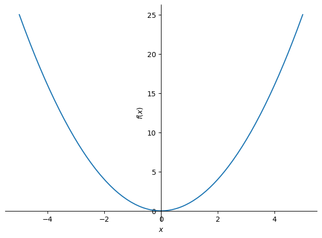
Let’s plot \(f(x^2)\) over \([-5,5]\),

graph = sy.plot(x**2, (x, -5, 5))

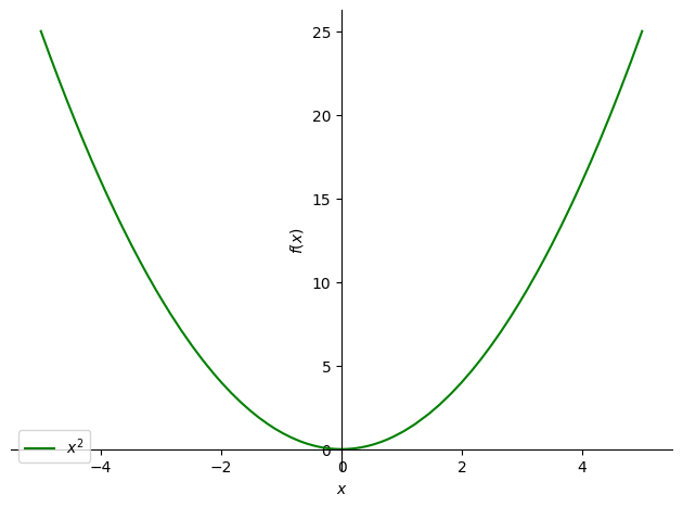
We can change the colour of the line and insert a legend for example,

graph = sy.plot(x**2, (x, -5, 5), line_color = 'green', legend ='True')

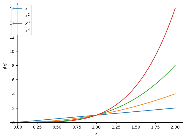
We can also plot multiple equations together,

multi_plot = sy.plot(x, x**2, x**3, x**4, (x, 0, 2), legend=True)

This is a small sampling of the sort of symbolic power SymPy is capable of, for more information access SymPy documentation.